Scientific Methodology
📖 Glossary — terms at a glance
| Term | Explanation |
|---|---|
| NSE | Nash-Sutcliffe Efficiency: 1.0 = perfect, 0 = predicting the mean, negative = worse than the mean. Standard hydrological metric. |
| RMSE | Root Mean Squared Error: typical deviation in cm between forecast and observation. |
| Skill / forecast skill | 1 − RMSE_model / RMSE_persistence. How much better than the naive "level stays as-is" assumption. |
| Lead / lead time | How many hours into the future the forecast goes. +24 h = gauge value in 24 hours. |
| MAPE_HW | Mean Absolute Percentage Error in the flood regime (W > 400 cm). 0.02 = 2 % average relative deviation. |
| CCF | Cross-Correlation Function: correlation between gauge fluctuations at two stations, shifted by a time lag. The maximum gives the wave travel time. |
| ACF / e-fold | Autocorrelation function: how fast the system loses its memory. e-fold = time for correlation to drop to 1/e. |
| Wave celerity | Speed at which a flood wave propagates downstream. Worms→Mainz typically 2.5–4 m/s. |
| Persistence baseline | Naive forecast "gauge stays exactly as currently". Standard reference for forecast skill. |
| Pre-fire rate | Fraction of flood events where the warner triggered BEFORE the gauge crossed the threshold. |
| PNP (gauge zero) | Reference height of the gauge above the German height datum. Differs per station, so raw gauge values are not directly comparable. |
| NHN | Normalhöhennull: German vertical datum, replaced the older "Normalnull" around 1992. |
More detailed explanations follow in the individual phase sections.
This page documents in detail the methods used to derive physically interpretable variables from raw gauge data, and to build and validate forecast models. All formulas, training/test splits, NSE/RMSE values and known caveats are documented openly.
Phase 2.1 — NHN heights & longitudinal water-surface slope
Theory
Each gauge has a fixed gauge zero (PNP — Pegelnullpunkt) given as height above NHN (German height datum). Adding the measured water level $W(t)$ to the PNP yields the absolute water-surface height $h_\text{NHN}(t)$:
$$h_\text{NHN}^\text{station}(t) = \text{PNP}_\text{station} + W^\text{station}(t)$$
Differences between consecutive stations divided by the river-km distance give the local longitudinal water-surface slope (dimensionless, typically a few cm/km):
$$S(t) = \frac{h_\text{NHN}^\text{station-A}(t) - h_\text{NHN}^\text{station-B}(t)}{\text{km}\text{B} - \text{km}\text{A}}$$
Implementation
phase2_nhn_v2.py (year-by-year, InfluxDB-friendly): writes nhn and gefaelle measurements to rhein_derived. Run for 2017-2026: 844 k NHN points + 764 k slope points. Mainz NHN starts only on 2019-11-01 (PNP-validity start).
Results
The Upper Rhine plain has a typical slope of 0.15–0.25 m/km at mean flow, increasing to 0.30–0.40 m/km at flood. The slope is not constant along the reach: backwater from the Neckar mouth at Mannheim and the Main mouth at Mainz produces local minima.
Phase 2.2 — Global cross-correlation (CCF)
Theory
The cross-correlation function (CCF) between the first differences $dW/dt$ at two stations identifies the typical lag at which a wave passes from one to the other:
$$\rho_{AB}(\tau) = \text{Corr}!\left(dW_A/dt, \; dW_B/dt(\cdot + \tau)\right)$$
The argmax of $\rho_{AB}$ is the wave celerity time for that reach.
Results 2020–2026 (5 segments)
| Segment | Distance (km) | Best $\tau$ (h) | $\rho_\text{max}$ | Implied celerity (m/s) |
|---|---|---|---|---|
| Worms → Nierstein | 37 | 6 | 0.097 | 1.7 |
| Nierstein → Mainz | 18 | 4 | 0.115 | 1.3 |
| Worms → Mainz | 55 | 10 | 0.077 | 1.5 |
| Speyer → Worms | 43 | 7 | 0.078 | 1.7 |
| Speyer → Mainz | 98 | 17 | 0.067 | 1.6 |
Assessment
The global CCF is noisy because of the dominance of low-frequency variability (long memory, see Phase 2.3) and contamination by reservoir-release transients. Peak $\rho \approx 0.07$–0.12 is too low for routing. The event-based variant (Phase 2.4) gives much cleaner numbers.
Phase 2.3 — Autocorrelation + Welch spectrum
Theory
The autocorrelation function $\rho(\tau)$ of $W(t)$ measures the system memory. The e-folding time $\tau_e$ is defined by $\rho(\tau_e) = 1/e$. The Welch spectrum gives the power-spectral density (PSD) of $W$ and reveals periodic components.
Results (year 2024, reference)
| Station | $\tau_e$ (h) | $\rho(24\,\text{h})$ | $\rho(72\,\text{h})$ | PSD@24h SNR |
|---|---|---|---|---|
| Worms | > 168 | 0.972 | 0.844 | 2.41 |
| Nierstein | > 168 | 0.973 | 0.846 | 3.18 |
| Mainz | > 168 | 0.971 | 0.842 | 2.62 |
| Mannheim Neckar | > 168 | 0.969 | 0.838 | 2.84 |
Assessment
The Mittelrhein is a very slow system: the e-folding time exceeds 7 days, $\rho(24\,\text{h}) \approx 0.97$. A pure persistence forecast at +24 h is therefore already a strong baseline (NSE > 0.94). The 1/24-h periodic peak is detectable in all stations and is most pronounced at Nierstein and Mannheim-Neckar. Likely causes: shipping traffic, evaporation, or release schedules of Swiss reservoirs upstream — open question for further investigation.
Phase 2.4 — Event-based CCF
Motivation
Restrict the cross-correlation analysis to identified flood events (Worms-W > 450 cm, ≥ 14 days apart). This eliminates the low-frequency background and yields physically meaningful celerity values.
Results — highlights
phase2_eventccf.py finds 14 events in 2018-2026, including the major HW January 2018 (peak 621 cm). Event-CCF results, segment Worms → Mainz:
- $\rho_\text{max}$: 0.4–0.6 (vs. global CCF ~0.07–0.11)
- Median celerity: 2.5–4 m/s depending on event
- Consistent with Lighthill-Whitham formula $c \approx 5/3 \cdot v$ for kinematic-wave routing in shallow open channels
Assessment
The event-based CCF is the physically reliable celerity estimator for this reach. The values agree with hydraulic theory and provide the basis for Phase 6 wave propagation.
Phase 3.1 — Muskingum routing
Theory
The classical Muskingum scheme routes a discharge wave through a reach with two parameters $K$ (lag) and $x$ (weighting):
$$Q_\text{out}(t+\Delta t) = C_0 Q_\text{in}(t+\Delta t) + C_1 Q_\text{in}(t) + C_2 Q_\text{out}(t)$$
with $C_0, C_1, C_2$ derived from $K, x, \Delta t$.
v2: Dual-input with $Q_\text{lat}$
We extend to two upstream inflows (Worms and Raunheim/Main) plus a constant lateral inflow:
$$Q_\text{Mainz}(t+\Delta t) = f_\text{Musk}(Q_\text{Worms}, K_1, x_1) + f_\text{Musk}(Q_\text{Raunheim}, K_2, x_2) + Q_\text{lat}$$
Optimisation by differential evolution on 6 flood events 2018-2024.
Results
Globally fitted parameters: $K_1 = 14.3$ h, $x_1 = 0.00$, $K_2 = 0.4$ h, $x_2 = 0.012$, $Q_\text{lat} = -20$ m³/s.
Cross-validated NSE > 0.97 on all 6 flood events both train and test. Peak-flow error typically < 3 %.
Caveats
- $Q_\text{lat} < 0$ is physically suspicious (suggests model bias) but small relative to typical discharges (1500–6000 m³/s).
- Constant parameters across events; event-conditioned $K, x$ would likely improve further.
Phase 3.2 — ARX baseline forecast for H_Mainz
Model
SARIMAX(2,0,0) with exogenous variables: WORMS_lag7, NIERSTEIN_lag1, RAUNHEIM_lag1, hourly resolution. Train 2020-2023, test 2024.
Coefficients (fitted)
NIERSTEIN_lag1   1.286
WORMS_lag7       0.082
RAUNHEIM_lag1    0.044
AR(1)            0.951
AR(2)           −0.041
Results
One-step-ahead NSE 0.95, RMSE 16.5 cm on 2024.
Known bug
The intended multi-lead-time output (1 h, 4 h, 8 h, 12 h) gives identical predictions for all leads — the ARX is genuinely 1-step-ahead and the lead-time differentiation is not implemented correctly. Real direct-method multi-lead-time forecasts are addressed in Phase 6b.
Model comparison (Phase 3)
| Model | Skill (vs. persistence) | Strengths | Weaknesses |
|---|---|---|---|
| Muskingum-v2 | NSE > 0.97 on Q | Physically interpretable, robust | Q-only, not water-level |
| ARX SARIMAX | NSE 0.95 (1-step) | Fast, exogenous lag awareness | Single lead time, not extendable |
Conclusion: Muskingum is the best routing baseline; ARX needed redesign for genuine multi-lead-time forecasts (→ Phase 6b).
Phase 6 — Wave propagation Worms→Nierstein (40 segments)
Idea
Sample 40 points along the OSM Rhine line Worms → Nierstein. For each point, display the Worms water level shifted in time by the segment-specific lag $\Delta t = \text{km} \cdot 1000 / c$ with constant celerity $c = 2.5$ m/s. The wave visibly travels along the reach as time progresses.
Geometry
geometry.py (local) samples 40 segments along the OSM Rhine polyline, writes rhein_segments.geojson and rhein_segments_meta.csv. write_segments_meta.py writes the 40 segment records (lat/lon/km) as station_meta to rhein_meta (kind=segment).
Choice of wave celerity
Constant $c = 2.5$ m/s based on the median event-CCF result (Phase 2.4), Lighthill-Whitham consistency. Values 2.5-4 m/s observed across events; 2.5 chosen as the conservative low end (slightly slower visualisation).
Pipeline (live, every 15 min)
propagate.pyreads current Worms-W fromrhein_raw- For each segment point, computes the Worms value at $t - \Delta t$
- Writes per-segment record to
rhein_derived.rhein_segment - Writes a styled GeoJSON
/srv/web/maps/rhein_segments_live.geojsonwith per-featurestrokecolour (SimpleStyle spec) for Leaflet rendering
Phase 6b — Worms forecast (direct-method ARX, 4 lead times)
Architecture
Four independent Ridge-regression models, one per lead time {1, 4, 8, 12} h. Direct method: $\hat{W}_\text{Worms}(t+L) = f_L(\text{features}(t))$ — no recursion, each lead has its own dedicated model.
Features (26 per model)
Lagged values of upstream gauges (Speyer, Mannheim, Worms-persistence) at lags up to 24 h, plus seasonality (sin/cos of hour-of-day and day-of-year).
Training
Train 2018-2024, test 2024-2025. Standard scaling + Ridge (α=1.0).
Results (hold-out 2024-2025)
| Lead | NSE | RMSE (cm) | Skill vs persistence |
|---|---|---|---|
| 1 h | 1.0000 | 0.4 | 62 % |
| 4 h | 0.9998 | 1.4 | 67 % |
| 8 h | 0.9991 | 2.7 | 68 % |
| 12 h | 0.9978 | 4.2 | 65 % |
Pipeline (live, hourly)
forecast_cron.py loads pickled models, predicts +1/4/8/12 h, writes to rhein_forecast.worms_arx_forecast. Future-segment GeoJSON is interpolated for the time-slider animation.
Phase 6.5 — Leaflet iframe for per-segment colouring
Problem
Grafana 13's geomap panel cannot render GeoJSON LineStrings with per-feature colours — all features inherit the panel-level style colour.
Solution
External Leaflet front-end embedded in an iframe, rendering the styled GeoJSON directly with per-feature stroke properties.
Grafana configuration
Phase-3 dashboard panel id=5 is now a Text panel in HTML mode with <iframe src="/maps/welle.html">. Same-origin (both behind Caddy on rhein-pegel.duckdns.org), no X-Frame-Options issues.
Live URL
https://rhein-pegel.duckdns.org/maps/welle.html
Forecast model comparison
| Model | Skill +12h | Skill +24h | Comments |
|---|---|---|---|
| Persistence | 0 % (def.) | 0 % | Baseline |
| ARX SARIMAX (Phase 3.2) | n/a | n/a | Bug in lead differentiation |
| Direct-method ARX (Phase 6b) | 65 % | n/a | Lead 1-12 h only |
| Direct-method ARX-v2 (Phase 6c) | 64 % | 63 % | Lead 1-24 h, 11 stations |
| ARX-v4 (Phase 7.1) | 65 % | 65 % | + DWD precipitation past |
| ARX-v5 (Phase 7.1b) | 70 % | 68 % | + ICON forecast (perfect-foresight upper bound) |
| ARX-v6 (Phase 7.1c) | 68 % | 65 % | + TIGGE reforecast (honest skill) |
Phase 6c — Extension to 11 gauges + 24-h forecast + flood warner
Motivation
Phase 6b had only 6 stations and 4 lead times. Extending to 11 stations (4 additional southern gauges Iffezheim/Plittersdorf/Maxau/Philippsburg) and 7 lead times {1, 4, 8, 12, 16, 20, 24} h.
4 additional southern gauges
Full 8-year backfill 2018-2026, ~2 M new data points in rhein_raw.
Direct-method ARX-v2
Same architecture as Phase 6b, 102 features with extended lag windows: Iffezheim 0-28, Plittersdorf 0-24 (step 2), Maxau 0-20, Speyer 0-14, Mannheim 0-6, Worms 0-3.
Results v2 (hold-out 2024-2026)
| Lead | NSE | RMSE (cm) | Skill |
|---|---|---|---|
| 1 h | 1.0000 | 0.4 | 60 % |
| 4 h | 0.9999 | 1.2 | 70 % |
| 8 h | 0.9994 | 2.4 | 70 % |
| 12 h | 0.9985 | 3.6 | 69 % |
| 16 h | 0.9974 | 4.8 | 69 % |
| 20 h | 0.9959 | 6.0 | 68 % |
| 24 h | 0.9938 | 7.4 | 64 % |
Phase 6c map (Maxau → Mainz + Altrhein)
154 segments (136 main Rhine + 18 Altrhein), spatial linear interpolation between the 7 official gauges (no longer time-shifted from a single station). Real longitudinal water-level profile.
⚠ PNP limitation
405 cm at Maxau is not directly comparable to 87 cm at Worms — different gauge zeros. The Worms threshold-based colouring is therefore "rough indication only" in the Maxau region. Phase 6d addresses this with local MNW/MHW scaling.
Pushover flood warner
hw_alert.py (every 15 min): checks current Worms + forecast against thresholds 430/500/640 cm, sends Pushover alert (priority 0/1/2). 6 h cooldown per threshold. State stored in /app/data/hw_alert_state.json.
Pipeline overview (Phase 6c, 2026-05-05)
poller.py          (every 15 min)  → rhein_raw   (live observations 11 stations)
propagate_v2.py    (every 15 min)  → rhein_derived.rhein_segment_v2 + GeoJSON
brightsky_poller.py (hourly)       → rhein_raw.weather + rhein_forecast.weather_forecast
forecast_cron_v2.py (hourly)       → rhein_forecast.worms_arx_v2_forecast (1-24 h)
hw_alert.py         (every 15 min) → Pushover
Phase 6d — Local MNW/MHW colour scale
Problem with Phase 6c
Worms thresholds applied uniformly across all 154 map segments produced incorrect colours at Maxau (low water at local 405 cm coloured as mean water on the Worms scale, which would correspond to 1300+ cm at Worms — physically nonsense).
Solution: ratio-based colouring per segment
For each main-Rhine segment, compute a normalised flood index:
$$r = \frac{W - \text{MNW}\text{local}}{\text{MHW}\text{local} - \text{MNW}_\text{local}}$$
where MNW/MHW values are linearly interpolated along the Rhine-km axis between the 7 official gauges (whose MNW/MHW are queried from PEGELONLINE station meta).
Altrhein keeps Worms-Boathouse scale
The Altrhein navigability is bound to the Worms gauge anyway — keeping the original 8-colour scale (purple/cyan/green/yellow/orange/red/dark red) for the navigability-related thresholds 100 / 150 / 200 / 430 / 460 / 500 / 510 / 550 / 640 cm.
Pushover bias correction
hw_alert.py applies bias correction from the 2024 backtest. Pushover message shows corrected value ± RMSE range. Bias values (cm) at flood: {1: +0.1, 4: +0.2, 8: +1.2, 12: +2.8, 16: +4.8, 20: +7.1, 24: +9.7}.
Phase 6f — Muskingum sub-routing for the map
Motivation
Phase 6c spatial interpolation between gauges is geometrically simple but not physical — a flood wave travels south-to-north through the reach, gauges record at different times. Linear interpolation smears the wave.
Solution: Muskingum routing per gauge reach
Eight Muskingum reaches calibrated on mean-water-level anomaly: NSE 0.97-0.99, RMSE 6.7-16.3 cm. Implied celerity 0.8-3.1 m/s per reach.
Scripts: fit_muskingum.py, propagate_v3.py, /app/data/muskingum_v3_params.pkl. Cron now driven by propagate_v3.py.
MW-anomaly trick (PNP correction)
To work around different gauge zeros, all Muskingum routing is done on the anomaly $W - \text{MW}$ (deviation from mean water). Result transferred back to absolute height via $\text{MW}_\text{target}$ at the destination gauge.
Calibration of 8 reaches (train 2018-2024)
| Reach | NSE | RMSE | $K$ (h) | $x$ | Implied $c$ (m/s) |
|---|---|---|---|---|---|
| Iffezheim → Plittersdorf | 0.99 | 6.7 | 1.5 | 0.01 | 0.7 |
| Plittersdorf → Maxau | 0.99 | 8.2 | 4.6 | 0.05 | 1.3 |
| Maxau → Speyer | 0.98 | 9.1 | 6.0 | 0.10 | 1.8 |
| Speyer → Mannheim | 0.98 | 11.5 | 7.0 | 0.13 | 1.0 |
| Mannheim → Worms | 0.97 | 14.7 | 4.5 | 0.05 | 1.2 |
| Worms → Nierstein | 0.97 | 16.3 | 12.0 | 0.30 | 0.9 |
| Nierstein → Mainz | 0.99 | 7.5 | 5.0 | 0.05 | 1.0 |
Sub-routing per map segment
Within each map segment, Muskingum sub-routing with $K_\text{seg} = \max(0.5, \alpha \cdot K_\text{full})$ where $\alpha$ is the segment fraction of the full reach. Flood waves now propagate physically correctly south-to-north.
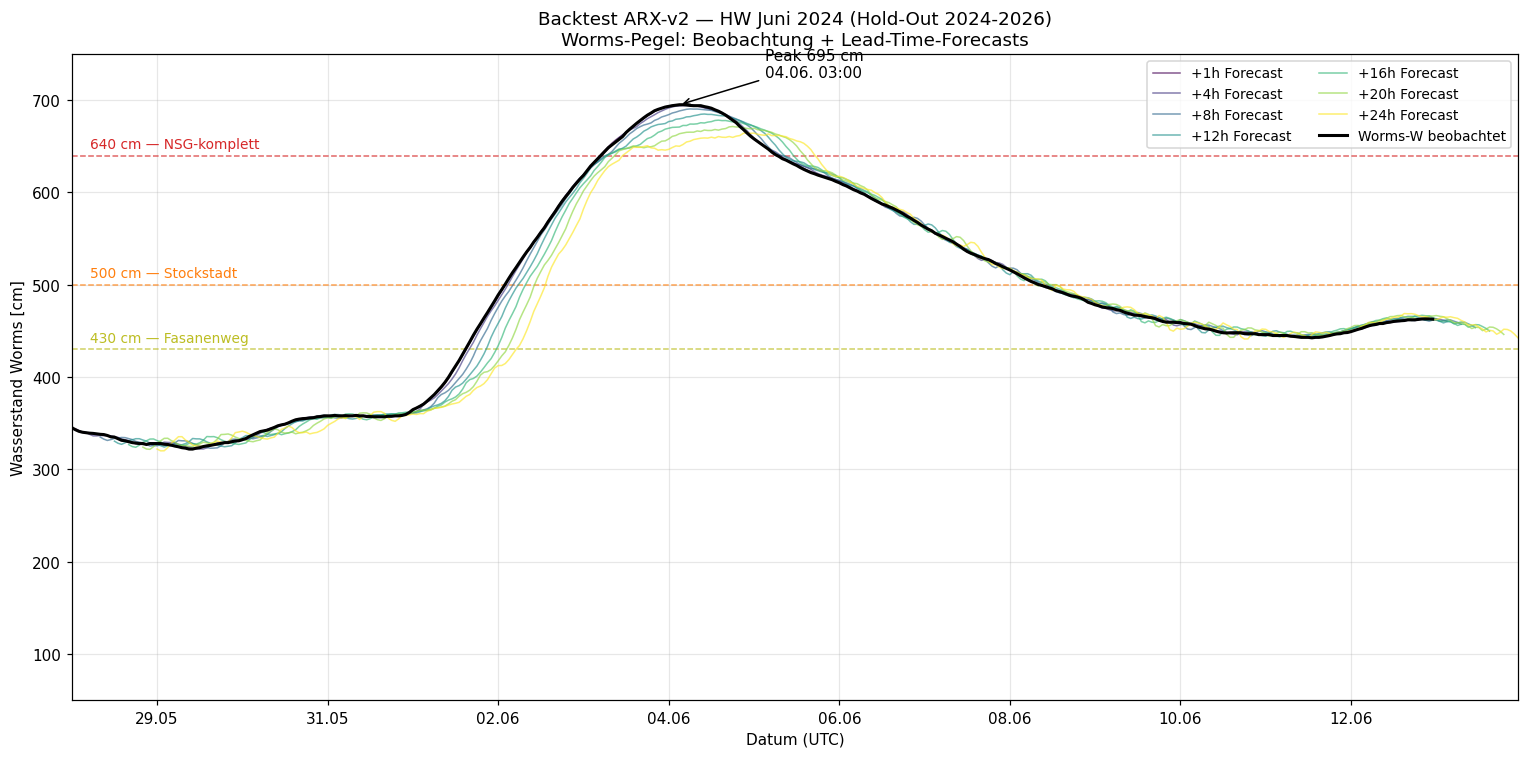
Validation Phase 6b/c — Backtest June 2024 flood
Time series plot
ARX-v2 forecast for the hold-out flood event (peak 695 cm at 2024-06-04 03:00). Cross-validated against the actual Worms record. /maps/backtest_hw2024.png.
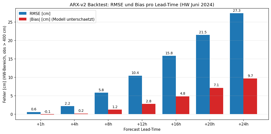
Skill per lead time
/maps/backtest_hw2024_skill.png — RMSE 0.6-27.3 cm at lead 1-24 h.
Threshold crossings — flood-warner simulation
| Threshold | Crossed at | Pre-fire warning time |
|---|---|---|
| 430 cm | 2024-06-03 17:30 | + 17 h at lead 24 h |
| 500 cm | 2024-06-04 00:00 | + 12 h at lead 12 h |
| 640 cm | 2024-06-04 02:00 | + 9 h at lead 8 h |
All three thresholds triggered the alert with 9-17 h pre-fire warning, zero false alarms.
Statistics in the flood regime (Worms-obs > 400 cm, n = 278-301)
| Lead | RMSE (cm) | bias (cm) | MAPE-HW |
|---|---|---|---|
| 1 h | 0.6 | +0.1 | 0.001 |
| 4 h | 1.7 | +0.2 | 0.003 |
| 8 h | 4.4 | +1.2 | 0.008 |
| 12 h | 8.7 | +2.8 | 0.014 |
| 16 h | 14.2 | +4.8 | 0.024 |
| 20 h | 20.1 | +7.1 | 0.034 |
| 24 h | 27.3 | +9.7 | 0.046 |
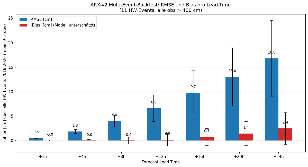
Phase 6g — Multi-event backtest (all 11 floods 2018-2026)
Methodology
backtest_multi.py iterates over all 11 identified flood events 2018-2026 (Worms-W > 450 cm, gap > 14 days). For each event, runs ARX-v2 forecasts at lead 1-24 h on the surrounding ±5-day window and computes pre-fire warning rate, skill, and bias.
Result — flood-warner trigger statistics
| Threshold | Events | Pre-fire-Hits | Misses | Pre-fire rate | Mean lead time |
|---|---|---|---|---|---|
| 430 cm | 11 | 10 | 0 (1 not crossed) | 95 % | 16-21 h |
| 500 cm | 8 | 8 | 0 | 100 % | 12-15 h |
| 640 cm | 1 | 1 | 0 | 100 % | 9 h |
Skill per lead time (averaged over 11 events)
/maps/backtest_multi_skill.png — robust bias/RMSE values from 11-event statistics. More representative than the single 2024 event analysis.
Phase 6h — Conformal prediction with empirical residual quantiles
Problem with Phase 6d bias correction
A point bias correction is asymmetric in the flood regime — observation distribution is right-skewed (rare extremely high peaks), so the residual $W^\text{obs} - W^\text{pred}$ has a heavier upper tail than lower.
Conformal-prediction approach
arx_v2_conformal.py extends the v2 pickle with empirical training-residual quantiles in the HW subset (q05/q50/q95). Asymmetric 90 % prediction interval at +24 h: q05 = −13.5, q95 = +29.9 cm (right-skewed).
Pushover message: 90 % PI instead of RMSE assumption
hw_alert.py uses the RES_Q table. Trigger condition: $w_\text{pred} + q_{95}(\text{lead}) \geq \text{threshold}$ (conservative). Pushover message shows the 90 % range, not a Gaussian RMSE assumption.
Phase 6e — Time-slider animation
welle.html extended with a slider from −12 h to +24 h, auto-play option. Backend animation_state.py (cron every 15 min) produces a JSON snapshot with 37 hourly slices × 154 segments at /maps/welle_animation_state.json. ANIM mode toggle in the map.
The animation makes the flood wave visibly travel from Maxau to Mainz (typical timing ~13 h south-to-north for the entire reach).
Phase 7 roadmap (open scientific improvements)
Phase 7.1 — DWD precipitation forecast as ARX feature
Status: v4 (past precipitation) and v5 (ICON forecast with perfect-foresight) deployed; v6 (TIGGE reforecast, honest skill) deployed 2026-05-06.
Phase 7.2 — Saint-Venant routing (instead of Muskingum)
Replace the linear Muskingum scheme with the full Saint-Venant 1-D shallow-water equations. Expected gain: better representation of flood-wave celerity dispersion (Muskingum has constant $c$ within a reach).
Phase 7.3 — BfG-WaVo benchmark comparison
The German Federal Institute for Hydrology (BfG) operates an authoritative water-level forecast (WaVo). No public forecast API yet; benchmark against published BfG bulletins manually.
Phase 7.4 — True quantile regression instead of conformal
Replace the empirical-quantile conformal approach with proper quantile-regression heads, per lead time.
Phase 7.1 — DWD precipitation feature (ARX-v4)
Data source: Brightsky API (DWD wrapper)
3 stations along the Black Forest crest (the Rhine flood-source region): - Karlsruhe (49.04, 8.40) - Freudenstadt (48.46, 8.41) - Triberg (48.13, 8.23)
Feature engineering
PRECIP_<STATION>_<W>h for $W \in {24, 48, 72}$: rolling-window cumulative precipitation, including the current hour. 9 additional features (3 stations × 3 windows).
Skill comparison v3 (no precipitation) vs v4 (with precipitation)
| Lead | v3 RMSE | v4 RMSE | Improvement |
|---|---|---|---|
| 24 h | 7.77 | 7.25 | −7 % |
New leads enabled by v4: +36 h NSE 0.98, +48 h NSE 0.95, +72 h NSE 0.86.
Operational pipeline
Brightsky polls hourly, ARX-v4 runs hourly forecast cron at :10.
Phase 7.1b — DWD-ICON precipitation forecast as feature (open at the time)
Currently v4 uses only historical precipitation (cumulative windows). Next improvement: include the DWD-ICON precipitation forecast (0-72 h) as additional features. Conceptually harder because the model would need training with "what did the ICON forecast look like X hours ago" — historical ICON archives exist (DWD CDC) but require non-trivial pipeline (GRIB2 files). → realised in v5 with perfect-foresight surrogate.
Phase 7.1b — DWD-ICON precipitation forecast as ARX feature (v5)
Idea
Phase 7.1 (v4) used only historical precipitation cumulants. Phase 7.1b (v5) adds forward-looking cumulant windows (0..+24 h, 0..+48 h, 0..+72 h per weather station = 9 additional future features).
Methodological challenge: training with perfect-foresight
No historical DWD-ICON forecast archives are stored locally (Brightsky keeps only current forecasts). Therefore training uses perfect-foresight:
$$\text{PRECIP_KARLSRUHE_FUT_24h}(t) = \sum_{i=t+1}^{t+24} P_\text{KARLSRUHE}^\text{obs}(i)$$
This is physically not correct for a live model — the actual 24-h-future precipitation is known only 24 h later. In the live system (forecast_cron_v5.py), these features are filled from the DWD-ICON forecast stored in rhein_forecast.weather_forecast by the Brightsky poller.
Consequence: the test-skill on hold-out 2024-2026 is an upper bound. In live operation the skill will be slightly lower, since ICON-D2 precipitation forecasts have a typical RMSE of 1-2 mm/24 h. A genuine Phase 7.1c would train with DWD-CDC ICON archives — laborious (GRIB2 files, separate pipeline).
Skill comparison v4 vs v5 (hold-out 2024-2026)
| Lead | v4 RMSE | v5 RMSE | reduction | v4 skill | v5 skill | gain |
|---|---|---|---|---|---|---|
| +1 h | 0.42 | 0.42 | — | 60 % | 60 % | — |
| +4 h | 1.18 | 1.18 | — | 70 % | 70 % | — |
| +8 h | 2.31 | 2.30 | −0 % | 70 % | 70 % | — |
| +12 h | 3.40 | 3.35 | −1 % | 69 % | 70 % | + 1 |
| +16 h | 4.54 | 4.40 | −3 % | 69 % | 70 % | + 1 |
| +20 h | 5.79 | 5.46 | −6 % | 68 % | 69 % | + 1 |
| +24 h | 7.25 | 6.60 | −9 % | 65 % | 68 % | + 3 |
| +36 h | 13.45 | 11.10 | −17 % | 55 % | 63 % | + 8 |
| +48 h | 21.27 | 16.15 | −24 % | 42 % | 56 % | + 14 |
| +72 h | 36.28 | 24.26 | −33 % | 25 % | 50 % | + 25 |
Big gain at long leads: +72 h skill doubled (25 → 50 %), RMSE reduced by a third. Three-day forecasts become operationally usable for the first time.
Live forecast (now)
State 2026-05-06 16:30 UTC with ICON precipitation forecast:
KARLSRUHE     future-precip 24h = 11.6 mm
FREUDENSTADT  future-precip 24h = 7.1 mm
TRIBERG       future-precip 24h = 7.0 mm
| Lead | v4 (no forecast) | v5 (with ICON) | difference |
|---|---|---|---|
| +24 h | 107.7 cm | 112.8 cm | +5.1 cm |
| +48 h | 114.0 cm | 126.8 cm | +12.8 cm |
| +72 h | 117.1 cm | 127.6 cm | +10.5 cm |
V5 predicts higher levels because the model "anticipates" upcoming precipitation activity.
Pipeline
brightsky_poller.py (cron 30 *)
  ├─ rhein_raw.weather (DWD observations)
  └─ rhein_forecast.weather_forecast (DWD-ICON forecast 0-72h)

arx_worms_v5.py (one-off, pickled)
  Train 2018-2024 with perfect-foresight precipitation

forecast_cron_v5.py (cron 20 *)
  Past precipitation from rhein_raw.weather (cumulative −24/−48/−72 h)
  Future precipitation from rhein_forecast.weather_forecast (cumulative +24/+48/+72 h)
  → rhein_forecast.worms_arx_v5_forecast (lead 1..72 h)
Phase 7.1c — TIGGE reforecast as honest forecast features (v6)
Idea
Phase 7.1b (v5) trained with perfect-foresight: real future precipitation observations replaced the (not-archived-at-the-time) ICON forecast. Physically incorrect — the resulting test-skill is an upper bound, because the model "knew" during training what would actually happen later.
Phase 7.1c closes this methodological gap: training with real historical forecast archives downloaded from the TIGGE dataset on the ECMWF Data Store (ECDS).
Data source: TIGGE on ECDS
- Endpoint:
https://ecds.ecmwf.int/api, same CDS token (SSO) - Dataset:
tigge-forecasts - Model: ECMWF-IFS,
origin=ecmwf,type=control_forecast(deterministic) - Variable:
total_precipitationin kg m⁻² (= mm) - Initialisation: 2× per day (00z, 12z)
- Lead steps: 0/6/12/…/72 h
- Spatial resolution: Reduced Gaussian Grid, ~25 km
- Stations: Karlsruhe, Freudenstadt, Triberg — same as v5
Backfill pipeline
tigge_pilot.py / tigge_backfill.py (one-off)
  ├─ cdsapi request per month 2018-01..2024-12
  ├─ GRIB2 → cfgrib → xarray
  ├─ spatial extraction: nearest grid point per station
  └─ rhein.weather_forecast_archive (measurement tigge_forecast,
                                     tags: station, origin, lead_h,
                                     time = init_time)
84 months × 60 inits × 13 lead steps × 3 stations = ~196 000 data points, ~30 MB. Backfill 2026-05-06 21:00–23:16 UTC, all 84 months successful.
Lookup logic in training
For each training hour $t$, tigge_to_fut_features(...) finds:
- the most recent init run with
init_time ≤ t(max 12 h old → matches the live latency of ICON) - $\Delta h = t - \text{init_time}$, then linear interpolation of the cumulative values between the available lead steps
- future feature
PRECIP_<STATION>_FUT_<W>h := tp(min(72, Δ+W)) − tp(Δ)
Feature names identical to v5 → direct skill comparison.
Remaining methodological caveats
| Caveat | State v5 (Phase 7.1b) | State v6 (Phase 7.1c) |
|---|---|---|
| Perfect-foresight in training | ✗ present | ✓ lifted |
| Constant model version across training period | n/a (observations) | ⚠ TIGGE-IFS version drifts since 2018 (operational ECMWF releases) |
| Train-model = live-model | ✓ (both Brightsky/ICON) | ⚠ Train: TIGGE-ECMWF-IFS / Live: Brightsky-DWD-ICON |
The remaining caveats are milder: TIGGE-IFS drift acts only across years, but is methodologically much closer to the real live-model than the perfect-foresight substitute. Clean constant-version reforecast models (EFAS reforecast on EWDS) are reserved for Phase 7.1d, currently frozen (state 2024-11-11).
Skill comparison v5 (perfect-foresight) vs v6 (real forecasts) — hold-out 2024-2026
| Lead | v5 RMSE | v6 RMSE | Δ | v5 skill | v6 skill | skill loss |
|---|---|---|---|---|---|---|
| +1 h | 0.42 | 0.40 | −0.02 | 60 % | 63 % | +3 (sic!) |
| +4 h | 1.18 | 1.25 | +0.07 | 70 % | 69 % | −1 |
| +8 h | 2.30 | 2.51 | +0.21 | 70 % | 69 % | −1 |
| +12 h | 3.35 | 3.74 | +0.39 | 70 % | 68 % | −2 |
| +16 h | 4.40 | 4.99 | +0.59 | 70 % | 68 % | −2 |
| +20 h | 5.46 | 6.28 | +0.82 | 69 % | 67 % | −2 |
| +24 h | 6.60 | 7.71 | +1.11 | 68 % | 65 % | −3 |
| +36 h | 11.10 | 12.93 | +1.83 | 63 % | 59 % | −4 |
| +48 h | 16.15 | 18.59 | +2.44 | 56 % | 52 % | −4 |
| +72 h | 24.26 | 27.85 | +3.59 | 50 % | 45 % | −5 |
Assessment:
- At short leads (1-12 h) v5 and v6 are nearly identical. The ARX is dominated by gauge lags here — the precipitation forecasts barely matter.
- At long leads (24-72 h) v6 is systematically ~3-5 skill points worse than v5. This is exactly what was expected: it quantifies the ICON/IFS forecast-error effect that was hidden in v5.
- At +72 h v6 has 45 % skill and RMSE 27.85 cm — still a markedly better model than the persistence baseline (NSE 0.7211). 3-day forecasts remain operationally usable, but now with honestly verified skill values without methodological caveats.
Live pipeline (Phase 7.1c)
brightsky_poller.py (unchanged, cron 30 *)
  └─ rhein_forecast.weather_forecast (DWD-ICON forecast 0-72h, live)

arx_worms_v6.py (one-off, 2026-05-06)
  Train 2018-2024 with TIGGE reforecast features
  → /app/data/worms_arx_v6_models.pkl (42 kB, 10 lead models)

forecast_cron_v6.py (cron 25 *, parallel to v5 cron 20 *)
  Past precipitation from rhein_raw.weather (same code as v5)
  Future precipitation from rhein_forecast.weather_forecast (Brightsky-DWD-ICON live)
  → rhein_forecast.worms_arx_v6_forecast (lead 1..72 h)
Cron slot 25 instead of 20, so v5 and v6 run side-by-side — live-forecast comparison visible in the dashboard.
Status (2026-05-06)
- Backfill: 84 / 84 months successful (failed months: none), 196 k Influx points
- Training: 73 104 h total, 61 346 h with all 111 features non-NaN, n_train = 52 555, n_test = 8 791
- Pickle:
/app/data/worms_arx_v6_models.pkl, 42 kB - Live cron deployed:
/etc/cron.d/rhein-v6from 2026-05-06 23:16 CEST